Simulation of Electrical Machines

The brief

Two machines, opposite directions. The first already existed: a 1.5 kW, six-pole interior permanent-magnet synchronous machine — the WONDER IPMSM — sitting in a lab at KTH with a nameplate and nothing else. The task was to rebuild it in software from its geometry alone and recover the electrical parameters the nameplate only summarizes. The second machine didn’t exist at all: a 1.5 kW, four-pole squirrel-cage induction motor to be designed from base specifications, geometry and equivalent circuit synthesized from scratch.

One is inference — take a real machine apart and explain it. The other is synthesis — start from a torque target and a voltage and build a machine that hits them. Doing both, in the same term, is what made the course worth writing up.

Reverse-engineering the IPMSM

Before any simulation, the machine had to be measured. The rotor and stator were sectioned so their cross-sections could be dimensioned directly — slot heights, tooth widths, the buried-magnet pocket geometry, the bridges that hold the magnets against centrifugal load.

Photograph of the physical IPMSM rotor sectioned across its axis, resting on a workbench in front of the machine's sectioned stator and its finned black housing. The cut face shows the near-hexagonal rotor lamination stack with the buried permanent-magnet pockets and their retaining bridges visible as dark slots around the perimeter. — The real rotor, cut across its axis: a near-hexagonal lamination stack with buried permanent-magnet pockets and the thin bridges that retain them. This cross-section is the geometry the whole model was built from.

Photograph of two IPMSM stator sections clamped and cut on a metal bandsaw, coolant pooled on the machine bed. Each section shows the 36-slot stator lamination stack with copper conductors packed into the slots, wrapped in a finned aluminium housing. — The 36-slot stator sectioned on the bandsaw — copper packed into every slot. A simulation project, but it started with hardware on a saw table.

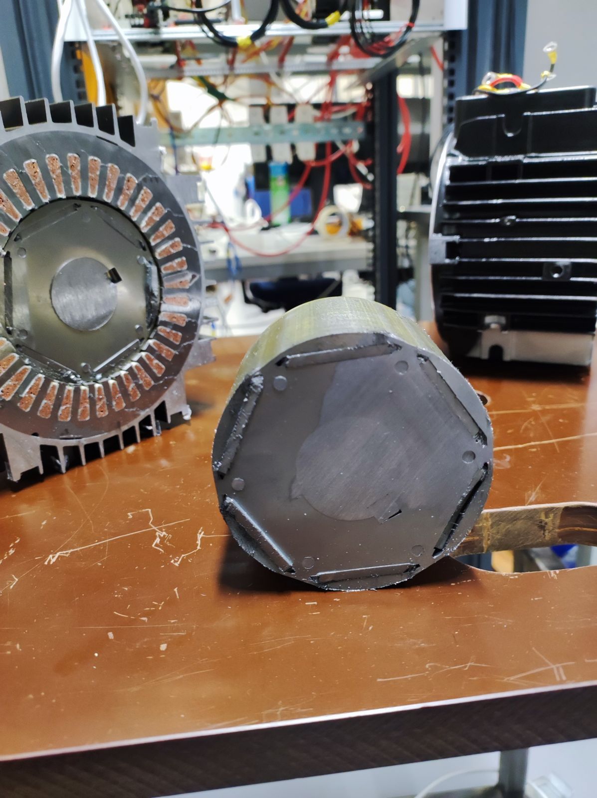
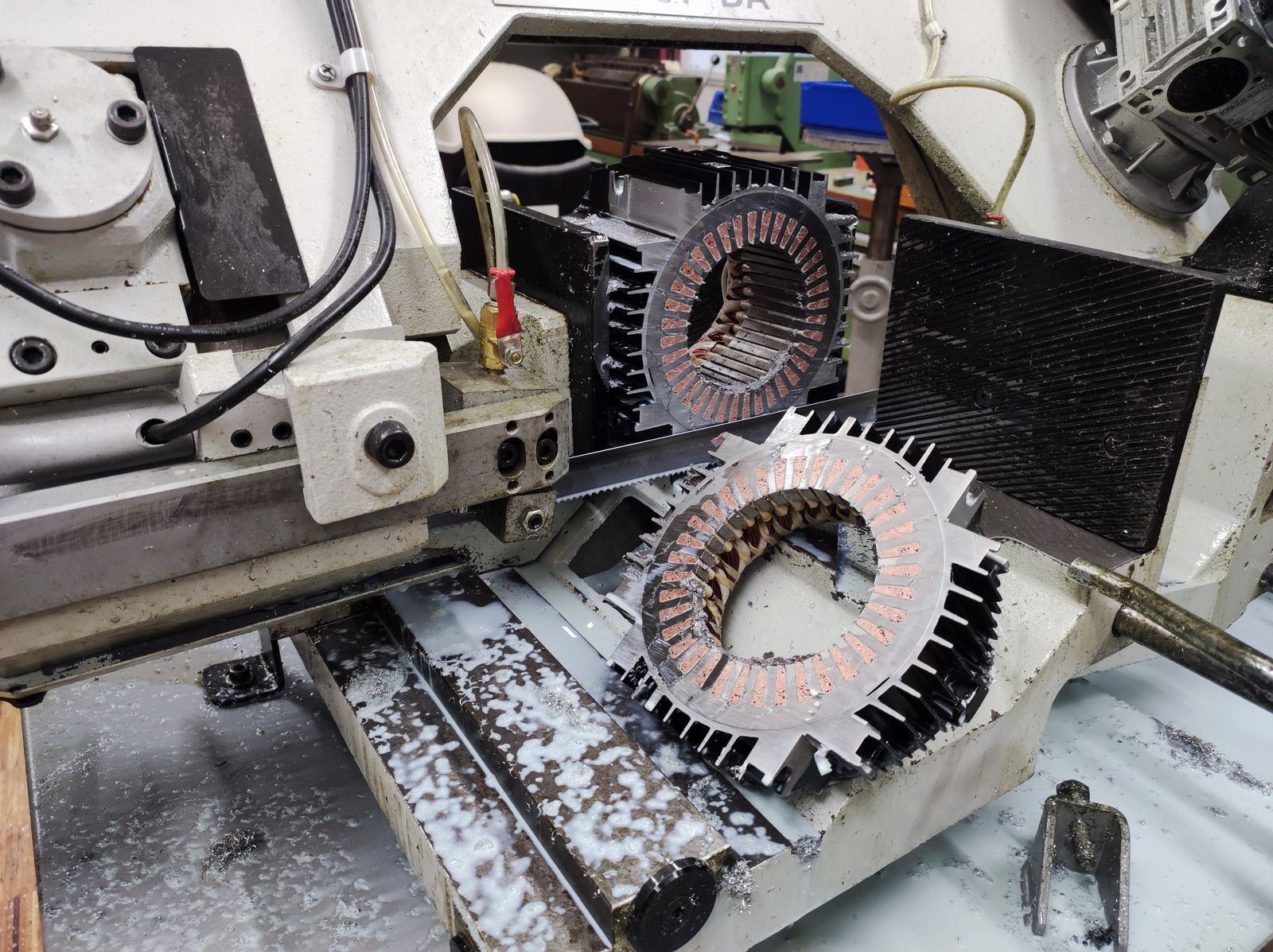
A simulation is only as honest as the geometry underneath it. Measuring the real laminations first — not trusting a datasheet drawing — is what let the extracted parameters land on the nameplate later.

From those measurements the machine was rebuilt in FEMM: 36 stator slots, six poles, two slots per pole per phase, a 65 mm active length, and the full buried-magnet rotor pocket with its wings and bridges. The stator winding was laid in as a two-layer, short-pitched three-phase distribution.

The first parameter fell out analytically. Phase DC resistance was computed from the total conductor length per phase — active length plus the end-turn arcs and stick-out beyond the core — giving 93.229 m of conductor and, at 20 °C, a phase resistance of 2.3600 Ω. That matched the laboratory measurement exactly, which was the first sign the geometry was right.

Automating FEMM

Everything past resistance needs a field solution, and not one solution — hundreds. Extracting flux linkage means stepping the rotor through a full electrical period. Extracting the d-q inductance maps means sweeping a rectangular grid of d- and q-axis currents. Finding the maximum-torque-per-ampere point means sweeping current angle at fixed magnitude. Each point is a fresh magnetostatic solve.

So the whole thing was driven from MATLAB through FEMM’s Lua interface: set the currents, solve, integrate, store, advance. A single run automates on the order of 500 magnetostatic solves without a hand touching the GUI. The heavy lifting is done by FEMM’s block-integral and line-integral commands — area-averaged magnetic vector potential over each slot for flux linkage, and Maxwell stress tensor over an air-gap contour for torque.

Getting the field quantities out correctly was the real work. Per-phase flux linkage came from the area-averaged vector potential A_z over each slot cross-section, weighted by the winding distribution — a ratio of two FEMM block integrals that already folds in the active length. A finer mesh was forced across the air gap specifically to keep the Maxwell-stress torque integration accurate, since that contour integral is where numerical noise shows up first.

The Park transforms were the part I refused to trust. Because every solve was expensive, a bug in the abc-to-dq mapping would have quietly poisoned a hundred data points before anyone noticed. So the transforms got their own test battery — round-trip abc→dq→abc, balanced-current sum-to-zero, amplitude invariance, and a check that the offset angle actually rotated the geometry — before a single current was injected.

Results

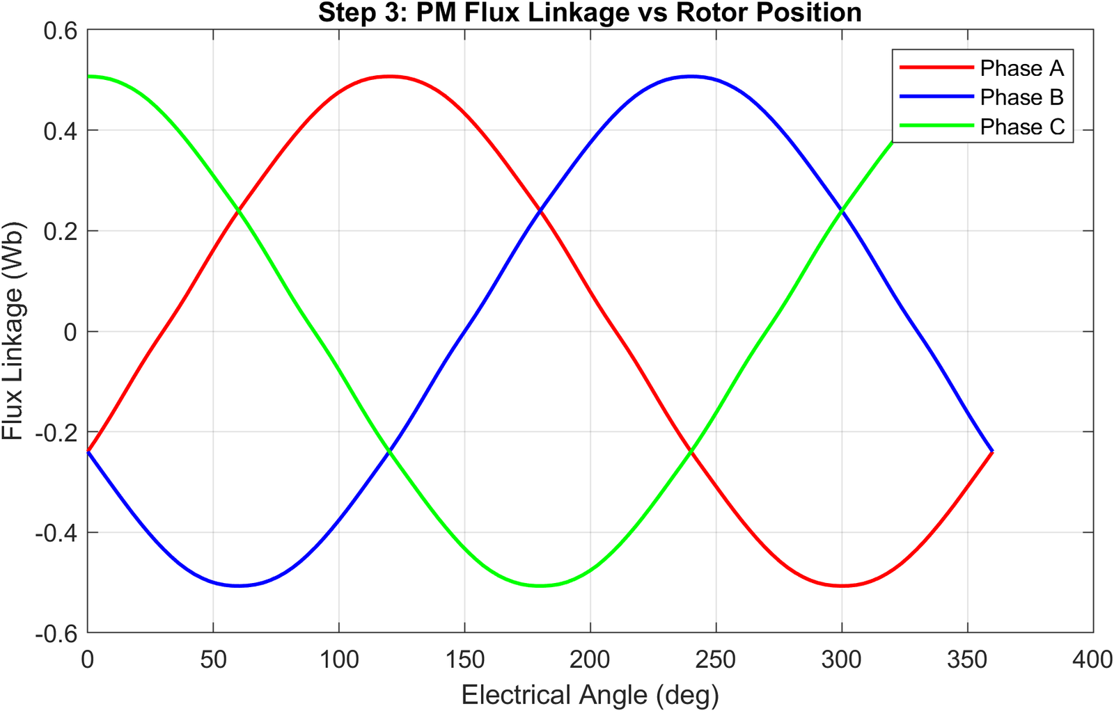
With the currents zeroed and the rotor stepped through an electrical period, the magnets are the only field source, and the per-phase flux linkage traces three clean balanced sinusoids.

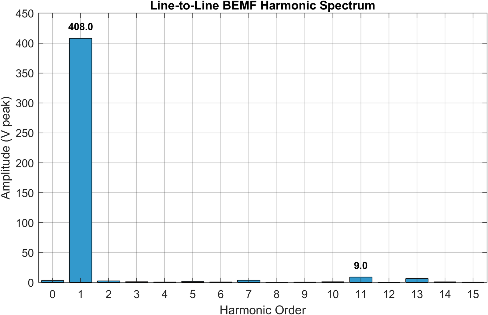
Line plot titled 'PM Flux Linkage vs Rotor Position' showing three sinusoidal curves — phases A (red), B (blue), and C (green) — each peaking near 0.51 Wb, spaced 120 electrical degrees apart, plotted over one electrical period from 0 to 360 degrees. — Permanent-magnet flux linkage over one electrical period: three balanced sinusoids peaking at 0.5068 Wb, spaced 120 electrical degrees apart. The peak of phase A also fixes the d-axis offset, 119.64 electrical degrees, that aligns every later Park transform.

Differentiating that flux linkage against rotor speed gives the back-EMF. Cross-checked three ways — an L2-norm RMS in the time domain, an FFT fundamental, and the mean-square — the line-to-line back-EMF came to 289.25 V RMS (289.06 V from the FFT fundamental), validating the 288 V nameplate. The spectrum is almost pure fundamental.

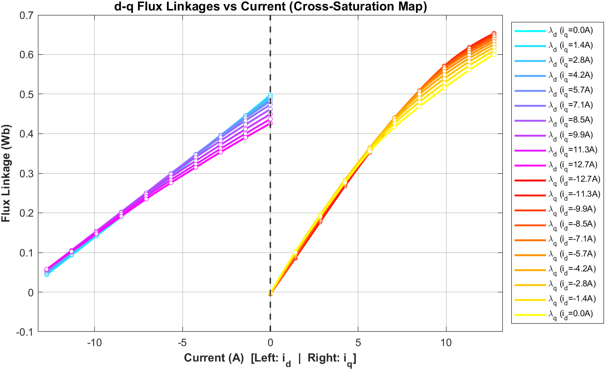
Bar chart titled 'Line-to-Line BEMF Harmonic Spectrum' showing amplitude in volts peak against harmonic order 0 to 15. The fundamental at order 1 dominates at 408 V peak; the largest higher harmonic is the 11th at 9 V, with all others near zero. — The back-EMF harmonic spectrum: a dominant fundamental with everything else in the noise. Total harmonic distortion of the line-to-line voltage, 2.83%.

Sweeping the full d-q current grid produces the flux-linkage maps that hold the machine’s saliency. The q-axis links more flux and saturates harder than the d-axis — the signature of an interior-magnet machine.

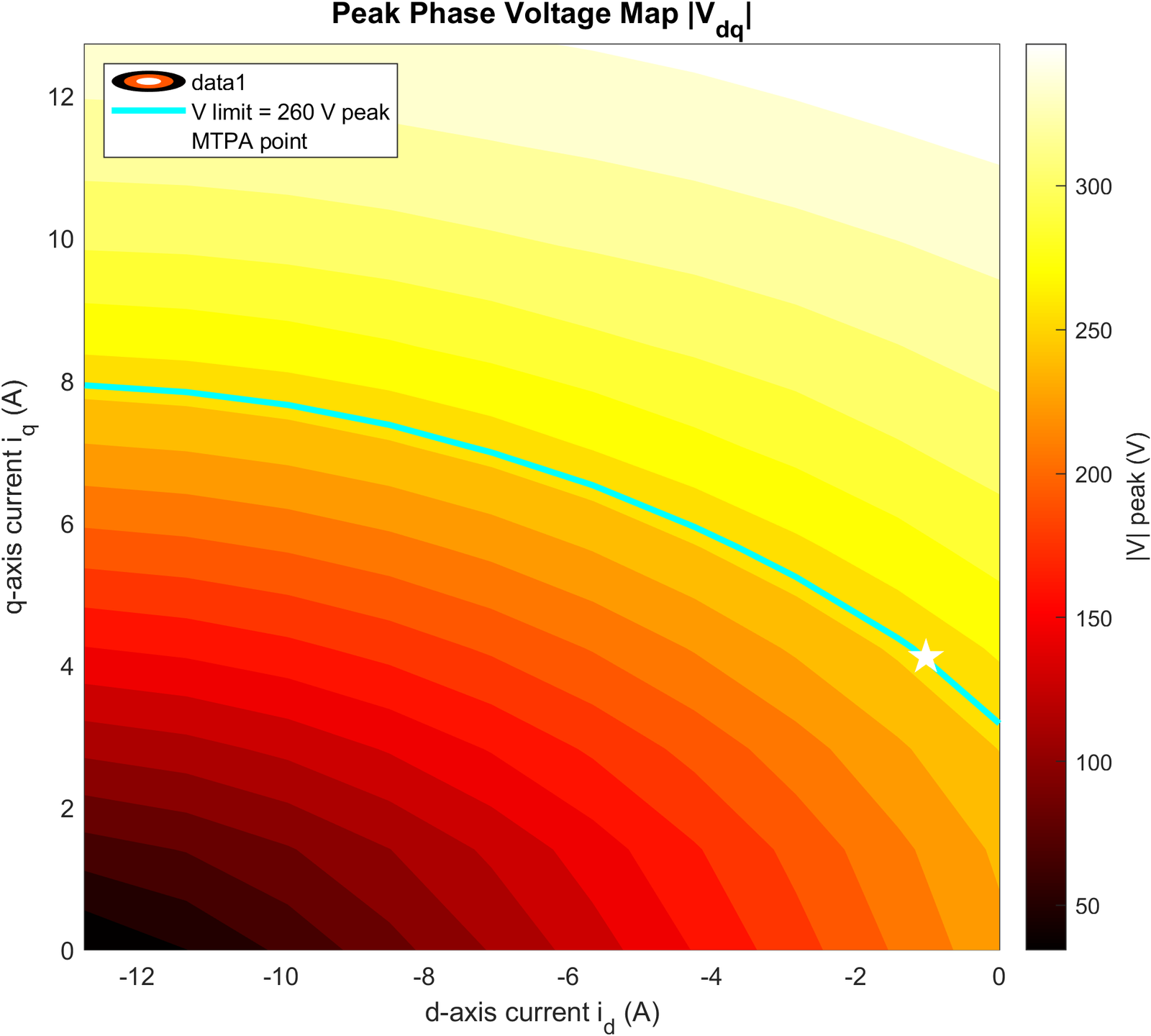
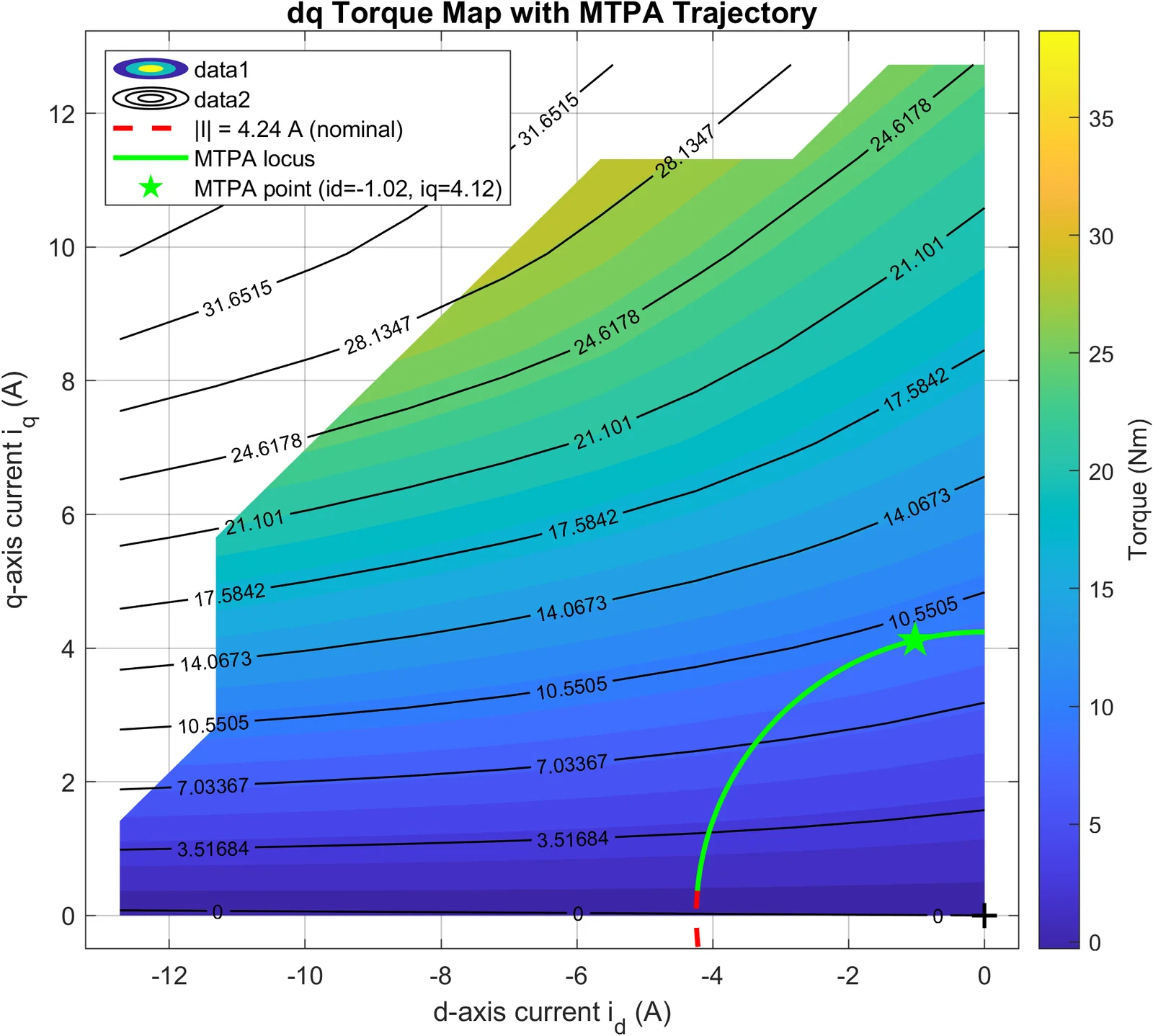
Plot titled 'd-q Flux Linkages vs Current (Cross-Saturation Map)' with two families of curves: on the left, d-axis flux linkage against negative d-axis current in cool colours; on the right, q-axis flux linkage against positive q-axis current in warm colours. The q-axis curves rise higher and bend over into saturation, the d-axis curves stay closer to linear. — d-q flux linkage against current. Incremental inductances taken along the axes give Ld = 36.34 mH and Lq = 58.80 mH — a saliency ratio Lq/Ld of 1.618, exactly what an IPMSM should show.

From the torque map, sweeping current angle at the nominal current magnitude locates the maximum-torque-per-ampere point: a current angle of 13.9°, drawing on reluctance torque that the nameplate never advertised.

Filled contour plot titled 'dq Torque Map with MTPA Trajectory' over the d-axis and q-axis current plane. Torque contours run from 0 to about 35 Nm; a green MTPA locus curves up from the origin to a green star marking the maximum-torque-per-ampere point at id = -1.02 A, iq = 4.12 A, where it crosses the dashed nominal-current circle of magnitude 4.24 A. — Torque across the d-q current plane, from Maxwell-stress integration. The MTPA point sits at id = -1.02 A, iq = 4.12 A: the negative d-axis current recruits reluctance torque, pushing the machine past its 9.6 Nm nameplate to a 10.21 Nm snapshot.

Running the optimal MTPA currents synchronously against the rotor gives the torque quality — and separately, with the windings off, the cogging torque from the magnets interacting with the slot openings.

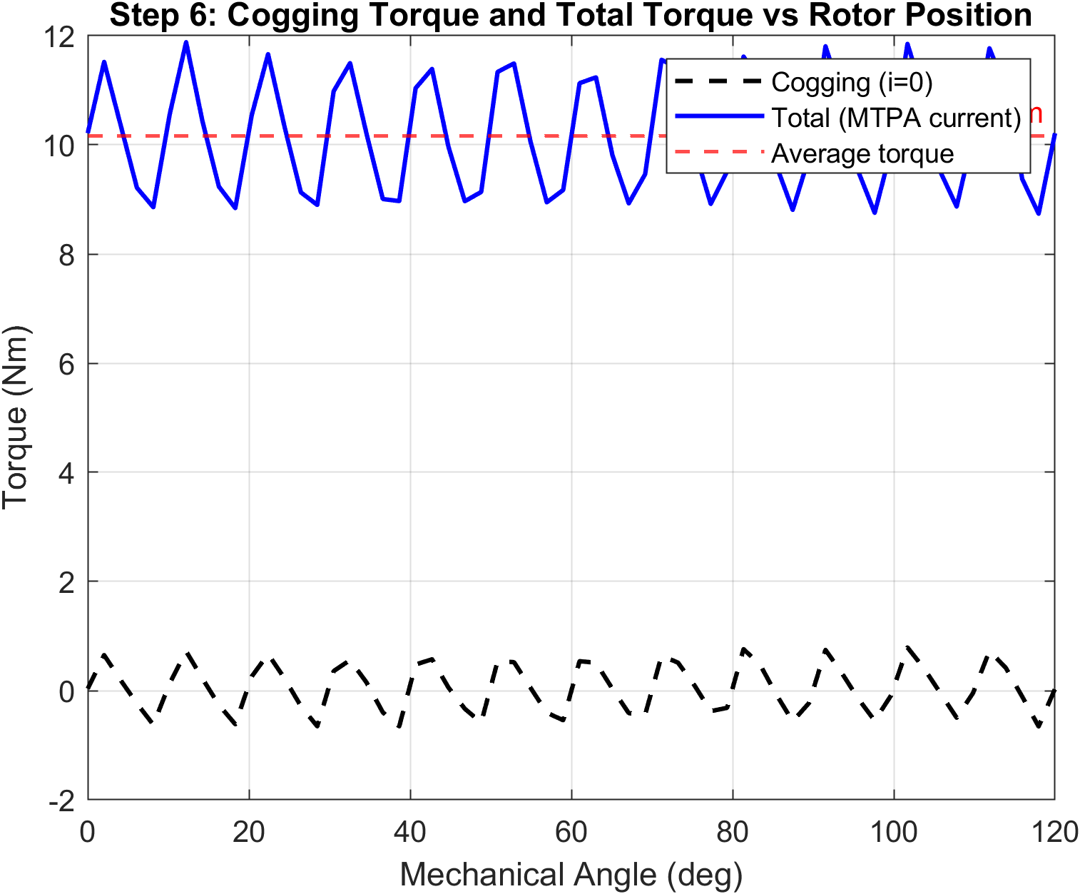
Line plot titled 'Cogging Torque and Total Torque vs Rotor Position' over 0 to 120 mechanical degrees. A blue curve for total torque under MTPA current oscillates between roughly 9 and 12 Nm around a red dashed average line near 10.2 Nm; a black dashed cogging-torque curve oscillates in a narrow band around zero. — Total torque under MTPA excitation against cogging with the windings off. Mean torque 10.17 Nm, peak-to-peak ripple 3.14 Nm (30.9%), cogging amplitude 1.45 Nm.

The closing check was independence: the same average torque, computed a second way from the d-q flux-linkage maps via the analytical dq torque equation, came to 9.69 Nm against the Maxwell-stress FEA value of 10.17 Nm — agreement within 4.6%. Two methods that share no intermediate results agreeing to within 5% is what confirms the Park transforms and the field integration are both sound.

Designing the induction motor

The second machine ran the process backwards. No hardware, no nameplate to recover — just a target: 1.5 kW, 400 V, 50 Hz, four poles, with an 85% efficiency floor and a 0.78 power-factor target. Following Lipo’s deterministic sizing algorithm, the job was to synthesize a full physical geometry and its T-model equivalent circuit from those specifications alone. The required electromagnetic torque set the anchor at 9.55 Nm.

The design didn’t converge on the first pass, and the reason it didn’t is the interesting part. Coupling the air-gap flux density straight to the stator-tooth density drove the air gap to about 0.875 T — deeply saturated. That saturation inflated the magnetizing current, suppressed the series turn count, collapsed the magnetizing reactance, and wrecked the power factor.

The fix was to stop treating one flux density as a slave of the other. Decoupling the air-gap flux density and pinning it at 0.75 T let the torque-producing current dominate, raised the turn count to 228, and pulled the magnetizing reactance back up to 127 Ω — which is what actually bought the power factor. The lesson is that the constraint you assume for convenience is often the one holding the whole design hostage.

From there a parametric sweep of volumetric current density fixed the stator split ratio and aspect ratio inside NEMA thermal bounds, landing a 105.4 mm bore in a 155 mm outer diameter, a 112.3 mm effective length, and 36 stator slots. The rotor was harder: the bar width was locked first by the rotor-iron flux-density limits, then a fixed-point iteration converged the bar depth, the stator-referred rotor resistance, and the rotor leakage reactance simultaneously — each one changing the others until they stopped moving. It settled on a 12.63 mm × 4.61 mm bar.

The finalized design meets every primary target, with nominal torque landing on the target within the precision carried in the calculation:

Metric	Target	Calculated
Nominal torque	9.55 Nm	9.55 Nm (error below 0.005%)
Output power	1500 W	1442 W (−3.84%)
Efficiency	85.3%	90.96% (+6.64%)
Power factor	0.780	0.783 (+0.33%)

Lessons

The two halves teach the same thing from opposite ends. Reverse-engineering the IPMSM, the discipline was distrust — expensive solves meant a silent bug in a transform could waste a hundred data points, so the transforms got tested before they got used, and every headline number got cross-checked a second way. Designing the induction motor, the discipline was noticing which assumption was doing the damage — the whole power-factor problem dissolved the moment the air-gap flux density stopped being coupled to the tooth density.

Both machines came down to the same habit: don’t trust the number until something independent agrees with it.